Research Interests
X-ray Absorption Spectroscopy (XAS) of Fe and S Species
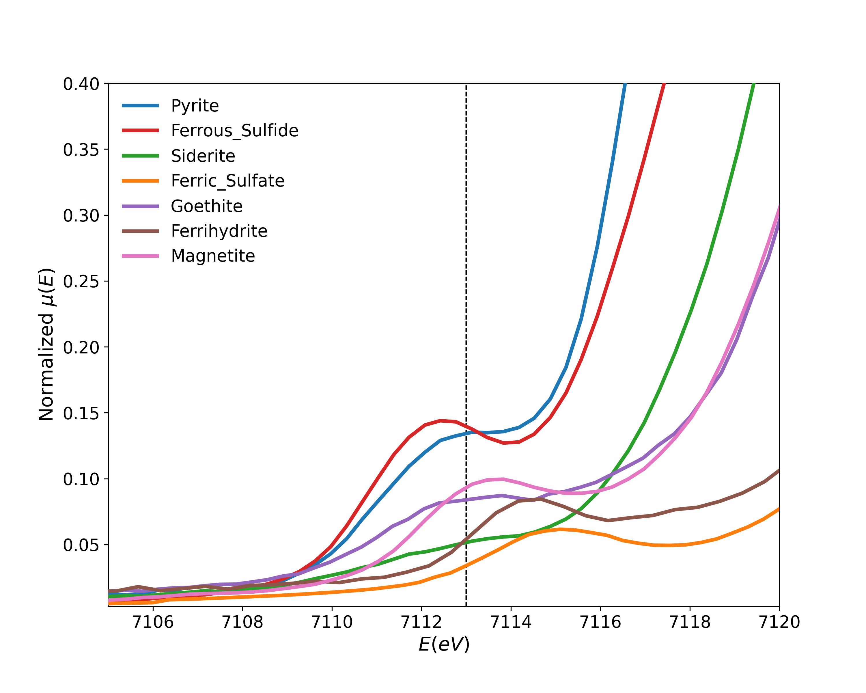
I started my postdoctoral work at the University of Saskatchewan by analyzing previously collected data from the SXRMB beamline at the Canadian Light Source (CLS). The data included standards and real samples with both Fe and S K-edge XAS measurements. Using Linear Combination Fitting (LCF), one can determine what standards constitute the measured samples. Fe K-edge XAS has an interesting pre-edge feature that can give a lot of information on the coordination environment of Fe atoms.
Fitting this pre-edge feature allows determining the Fe(II)/Fe(III) ratio:
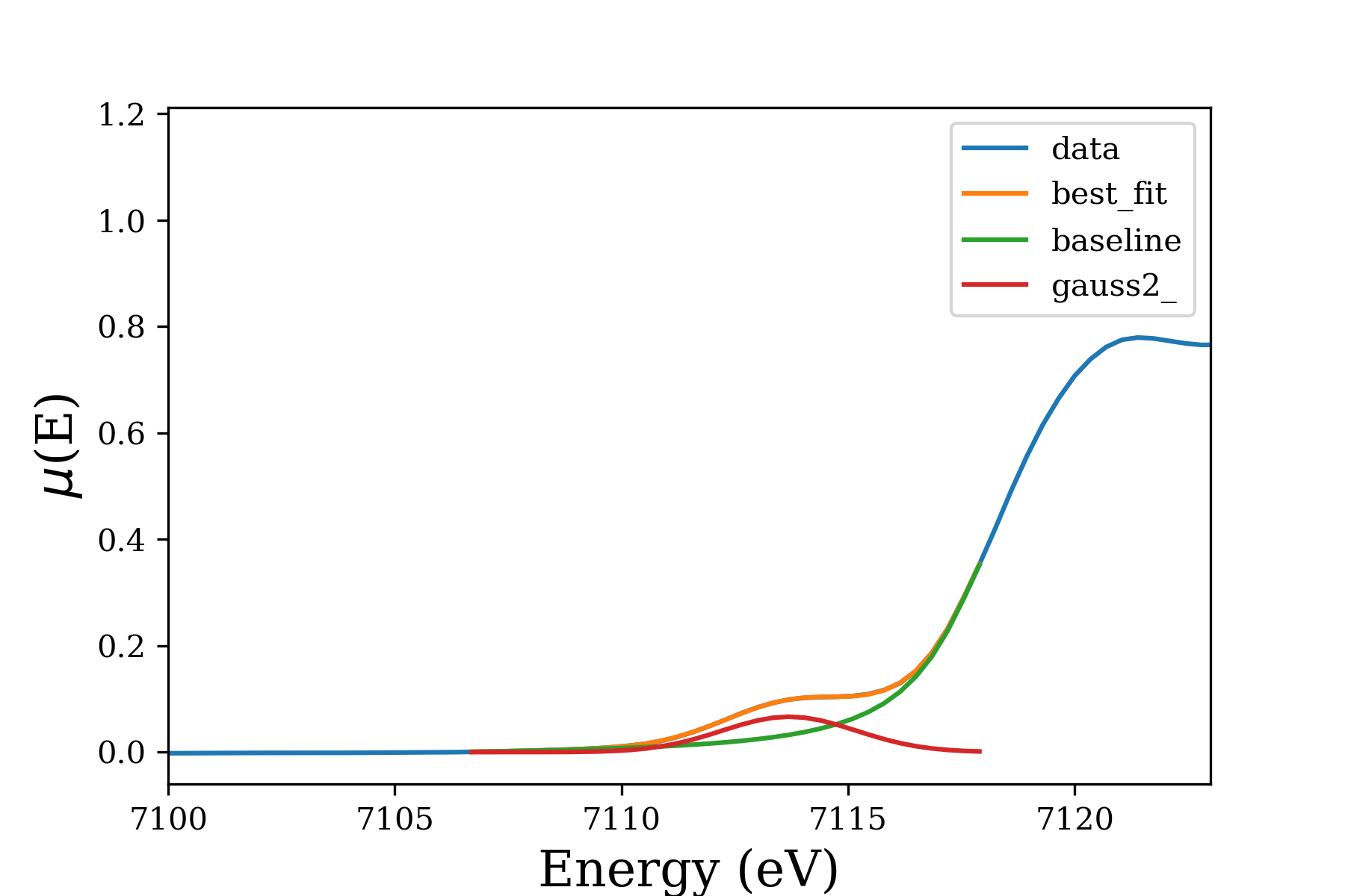
Here is a closer look at another fitted pre-edge feature:
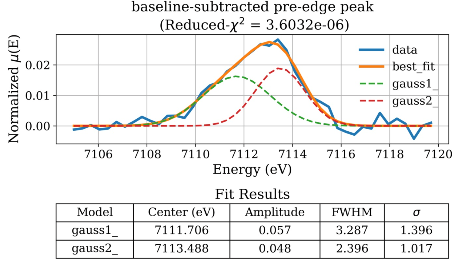
The pre-edge feature is due to \(1s \rightarrow 3d\) transition, and is sensitive to the local environment (e.g. oxidation state, symmetry) of Fe atoms. The pre-edge centroid position depends mainly on the oxidation state of Iron. However, its intensity is mostly dependent on the coordination environment around \(\ce{Fe}\) atoms.[1,2] The pre-edge is extracted from XANES spectra by using linear and Lorentzian functions to subtract the baseline, in the range of 7100–7120 \(\si{\eV}\). The isolated feature is fitted with Gaussian components. The addition of extra components is justified by improvements in reduced-\(\chi^2\). The fit results include Amplitude which represents the area of the unit-normalized peak.[3]
The \(\ce{Fe^{2+}}/\Sigma \ce{Fe}\) and \(\ce{Fe^{3+}}/\Sigma \ce{Fe}\) Ratios: Studies suggest that the individual pre-edge peaks between 7111.2–7112.2 \(\si{\eV}\) are mainly due to \(\ce{Fe^{2+}}\) \(\bigl(E_0^{\ce{Fe^{2+}}}\bigr)\) and peaks in the range of 7113–7114 \(\si{\eV}\) are mainly for \(\ce{Fe^{3+}}\) \(\bigl(E_0^{\ce{Fe^{3+}}}\bigr)\).[4,5] The fit centroid is area-weighted and is calculated according to the equation below:
\[ C = \frac{I^{\ce{Fe^{3+}}} \, E_0^{\ce{Fe^{3+}}} \;+\; I^{\ce{Fe^{2+}}} \, E_0^{\ce{Fe^{2+}}}} {I^{\ce{Fe^{3+}}} \;+\; I^{\ce{Fe^{2+}}}} \]
The determination of the oxidation state of \(\ce{Fe}\) using XANES is an indirect method and relies on calibration with wet chemical methods or Mössbauer spectroscopy data. There are several reports that utilize intensity ratios or centroid-based calibrations to determine the oxidation state of \(\ce{Fe}\) in samples.[4,6] For this study, the centroid-based calibration (shown below) reported by Knipping et al. will be used to calculate the \(\ce{Fe^{2+}}/\Sigma\ce{Fe}\) and \(\ce{Fe^{3+}}/\Sigma\ce{Fe}\) ratios. This equation is only valid when \(7111.9 < C < 7113.4\;\si{\eV}\), thus any sample with a centroid above the upper range is considered to be 100% \(\ce{Fe^{3+}}\).
\[ \frac{\ce{Fe^{2+}}}{\Sigma \ce{Fe}} = 1 \;-\; 0.5879 \times \bigl(C - 7111.9\bigr)^{1.2527} \]
[1] Yamamoto, T., et al. (2008).
[2] Wilke, M., et al. (2004).
[3] Newville, M. (2013).
[4] Knipping, J. L., et al. (2015).
[5] Alderman, O. L. G., et al. (2017).
[6] Wilke, M., et al. (2005).